6.1. Tutorial: Random Forest Classification
The following is a tutorial about the land cover classification using
the Random Forest algorithm in the Semi-Automatic Classification Plugin
(SCP).
Please note that the installation of the dependency scikit-learn is
required (see Plugin Installation).
It is assumed that you have already read the Basic Tutorials.
Following the video of the tutorial.
https://www.youtube.com/watch?v=2JU3XMkWdPo
6.1.1. Introduction
This tutorial describes how to perform the land cover classification of a multispectral image using the Random Forest algorithm. It is recommended to read the Tutorial 1: Basic Land Cover Classification before following this tutorial. We are going to identify the following land cover classes:
Water;
Built-up;
Vegetation;
Soil.
6.1.1.1. Download the Data and prepare the Band set
In this tutorial we are going to use a subset of Sentinel-2 Satellite
image, already converted to reflectance and clipped to the study area,
downloading a .zip file (which contains modified
Copernicus Sentinel data 2023).
Of course, this tutorial can be applied to any multispectral image.
Tip
For more information about how to download images, please read Tutorial 3: Downloading free satellite images, the Download product tab.
Download the .zip file from this
link 1
and extract the directory containing the image bands.
We must define the Band set which is the input image for
SCP classification.
Open the tab Band set clicking the button  in the
SCP menu or the SCP dock.
Click the button
in the
SCP menu or the SCP dock.
Click the button  to select the
 .tif files from the
extracted directory to the Band set tab.
Select Sentinel-2 in the
Wavelength list of the Band quick settings.
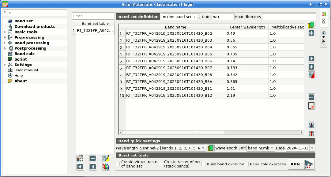
Definition of the band set
We can display the image in natural colors.
In the Working toolbar, click the list RGB= and select the
item 3-2-1.
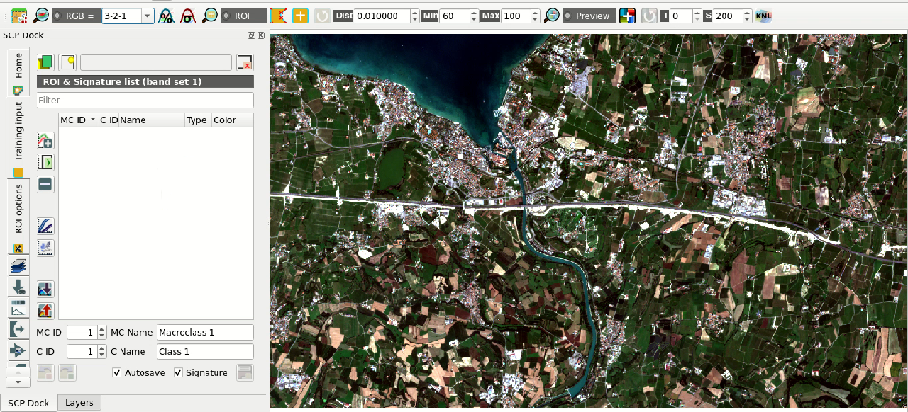
Color composite RGB=3-2-1
6.1.1.2. Create the ROIs
In general, we need to create a Training input
file in order to collect Training Areas (ROIs) to train the
classification algorithm.
In this tutorial, we are going to import a GeoPackage .gpkg file
containing polygons that we are going to import in a Training input
file.
Download the GeoPackage .gpkg file from this
link .
Tip
For more information about how to create the ROIs, please read Tutorial 1: Basic Land Cover Classification.
This GeoPackage .gpkg file includes the Macroclass IDs defined in the
following table, which is the classification system.
Of course, classes should be adapted to the classification objective.
Macroclass name |
Macroclass ID |
|---|---|
Water |
1 |
Built-up |
2 |
Vegetation |
3 |
Soil |
4 |
In the SCP dock select the tab Training input and click the
button  to create the Training input (define a name such
as
to create the Training input (define a name such
as training.scpx).
The path of the file is displayed and a vector is added to QGIS layers with the
same name as the Training input.
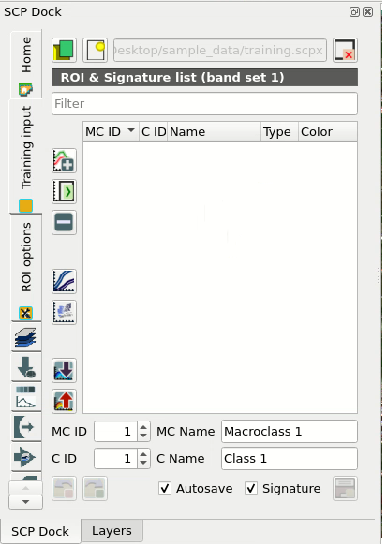
Definition of Training input in SCP
Now open the tool Import vector to import the GeoPackage
.gpkg file into the Training input.
First, in Select a vector select the path to the
GeoPackage .gpkg file.
Now we can select the vector field corresponding to MC ID field,
MC Name field, C ID field, and C Name field
which in this vector are macroclass_id, macroclass_name, class_id,
and class_name respectively.
Finally click Import vector  to import all the vector
polygons as ROIs in the Training input (this process can take a while).
Before running a classification (or a preview), set the color of land cover
classes that will be displayed in the classification raster.
In the ROI & Signature list, double click the color (in the column
Color) of each ROI to choose a representative color of each class.
Also, we need to set the color for macroclasses in ROI & Signature list.
to import all the vector
polygons as ROIs in the Training input (this process can take a while).
Before running a classification (or a preview), set the color of land cover
classes that will be displayed in the classification raster.
In the ROI & Signature list, double click the color (in the column
Color) of each ROI to choose a representative color of each class.
Also, we need to set the color for macroclasses in ROI & Signature list.
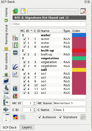
Imported ROIs in Training input
6.1.1.3. Create a Classification Preview and Random Forest parameters
We can now perform a Classification preview in order to assess the results before the final classification.
First, we need to select the classification algorithm
Random Forest.
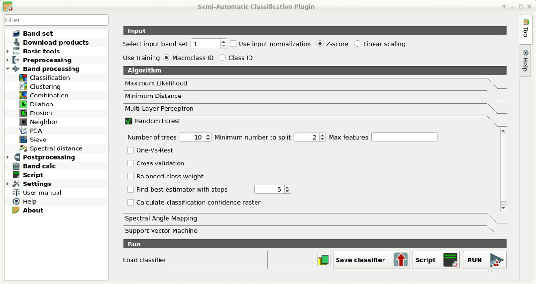
Open the tool Classification to set the input band set
(in this case 1), check Use  Macroclass ID,
and in Algorithm select the Random forest.
Macroclass ID,
and in Algorithm select the Random forest.
Selecting the algorithm
Tip
In case you defined the same Macroclass ID value for all the ROIs in
the Training input, you should check Use
Class ID.
Available parameters for Random forest are:
Number of treesthat sets the number of trees in the forest; this is one of the most important parameters because it defines the complexity of the forest, the higher the better but with the downside of increasing the computation time.Minimum number to splitthat sets the minimum number of samples required to split an internal node; in general it can be leaved 2 as default.Max featuresthat sets the number of features considered in node splitting; in general it can be leaved empty to consider all features in node splitting.
We can start with Number of trees set to 10 (the process should be rapid)
and in Classification preview set Size = 200; click the
button  and then left click a point of the image in the map.
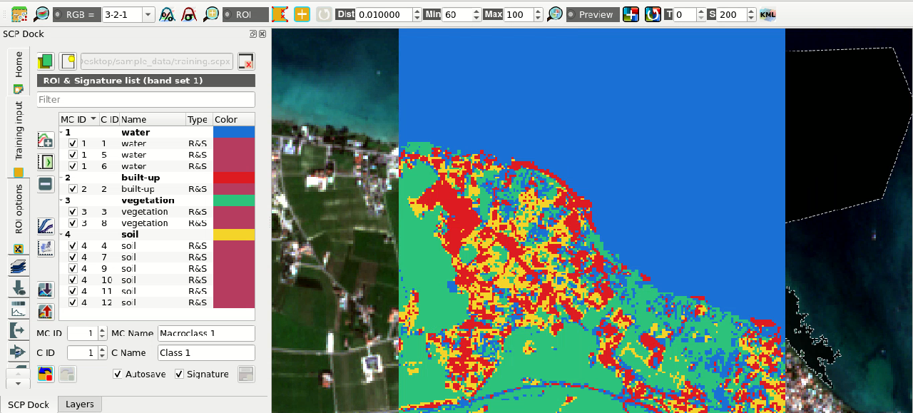
Classification preview displayed over the image
If we click again the button and then left click a point of the image
in the map, we should notice that the process is more rapid.
This is because the classifier is already trained, and directly used to
perform the classification.
We can increase Number of trees to 100, click the
button and then left click a point of the image in the map.
Now the process should take more time because changing the classification
parameters resets the classifier that needs to train again.
Tip
Generally, Number of trees should be at least 500 for good results.
Other interesting options are:
- One-Vs-Rest: if checked, the algorithm performs
One-Vs-Rest classification
which basically fits one classifier per class.
- Cross validation: if checked, perform cross validation
that is a function provided by
scikit-learnto avoid overfitting by splitting the training set intoksmaller sets (read more . In particular, the functionStratifiedKFold(with parameters n_splits=5, shuffle=True) is used to create 5 sets, each one containing approximately the same percentage of samples for each class as the complete set. This option can potentially increase significantly the computation time. - Balanced class weight: if checked, gives all classes
equal weight with a balanced weight that is computed inversely proportional
to class frequency in the training data.
- Find best estimator with steps: if checked, the
algorithm tries to find the best estimator iteratively with the defined
number of steps (the more the steps, the slower the process will be),
by changing the algorithm parameters.
The option Calculate classification confidence raster
is useful for the final classification output; if checked, in addition to the
output classification, a confidence raster is produced (each pixel represents
the confidence of the classifier in assigning the output class).
6.1.1.4. Create the Classification Output
Assuming that the results of classification previews are satisfactory, we can
perform the actual land cover classification of the whole image.
We can check the option
Calculate classification confidence raster to compute also the
confidence raster.
In Classification click the button Run  and define the path of the classification output file (.tif).
Tip
We can save the classifier for later use by clicking
Save classifier  .
.
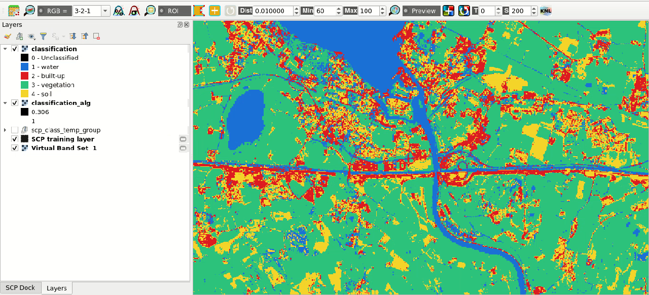
Result of the land cover classification
We can also analyze the confidence raster; higher values (i.e., near 1) represent pixels with high confidence, while lower values (i.e., near 0) represent pixels where the classifier is not well trained and more uncertain, therefore classification errors are expected.
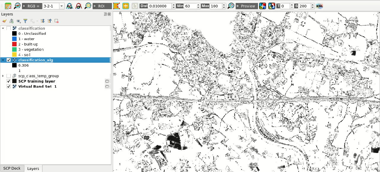
Confidence raster
Tip
It is recommended to analyze the pixels that have low confidence, and improve the classification by creating new ROIs or editing the existing ones.
We have performed a land cover classification using Random Forest algorithm. Other classification algorithms are described in other tutorials.